
By Ebenezer M. ASHLEY (PhD.) & Snows QUARM
In addition to the global economy, the economy of Ghana was randomly selected among the estimated two hundred and eighteen (218) global economies officially recognised by the World Bank (2021b) for the conduct of the current research. These global economies with recognition by the World Bank (2021b) comprise sovereign states or countries, dependencies and territories (Worldometer, 2021b).
Methodology
The current research was developed on the quantitative approach to scientific inquiry. Specifically, cross-sectional design, an example of survey design, was adapted and applied to the research. This design allowed the researcher to gather relevant research data over a specific time frame (Ashley, Takyi & Obeng, 2016; Creswell, 2009; Frankfort-Nachmias and Nachmias, 2008). Data required for the conduct of the current research were obtained mainly from secondary sources. These included text books, peer-reviewed articles published in journals, gray literature and newspaper publications. Other sources were Google Search Engine including MacroTrends; and databases of the World Bank, among other significant sources.
Respective data on annual global GDP growth rates and annual changes in global economic growth rates from 1961 through 2020; annual global inflation rates and changes in annual global inflation rates from 1981 through 2020; and respective data on Ghana’s annual GDP values from 1960 through 2020; annual GDP growth data from 1961 through 2020; annual inflation values and changes in annual inflation values from 1965 through 2020 were collected and used in the research.
The foregoing data formed the basis of the computation and application of the following annual averages to the current research: annual average inflation rate; annual average GDP growth rate; annual average GDP; annual average population; annual average population increase; and annual average GDP-to-annual average population ratio. Each of these averages was computed to reflect each political administrative period (both military and democratic) within the Ghanaian economy from 1960 through 2020. Specifically, the computed averages reflected the following periods: 1960 – 1965; 1966 – 1969; 1970 – 1971; 1972 – 1979; 1980 – 1981; 1982 – 1992; 1993 – 1996; 1997 – 2000; 2001 – 2004; 2005 – 2008; 2009 – 2012; 2013 – 2016; and 2017 – 2020.
Available data on Ghana’s annual GDP growth rates (first dependent research variable) extended to 1961 (MacroTrends, 2020a; World Bank, 2021d). However, the data’s application to the main statistical analysis was limited to 1965 to commensurate with the “earliest” available data accessed on Ghana’s annual inflation rates (first independent research variable) from MacroTrends (2020b).
Although available data on annual global GDP growth rates (second dependent research variable) extended to 1961 (MacroTrends, 2021b), the data’s application to the main statistical analysis was limited to 1981 to reflect the earliest available data accessed on annual global inflation rates (second independent research variable) from MacroTrends (2021c) during the research period. Descriptive statistics test conducted on Ghana’s annual GDP growth rates and presented in Figure 1 involved full complements of the available data from 1961 through 2020 as presented in Table 1; and Figures 3 and 4.
Analytical Tools
Descriptive statistics and regression models were used to describe the research variables; and to evaluate their behaviour over the stated time frame on GDP growth. Measures such as the mode, mean and median were used to identify desired average of the observations and to summarise the research data; while standard deviation and range were employed to describe the extent of dispersion about the central tendency (Ashley et al., 2016; Creswell, 2009; Frankfort-Nachmias & Nachmias, 2008). Specifically, these measures were used to describe trends in annual inflation and economic growth rates during the research period.
Research Variables
As affirmed in the preceding section, the independent research variable was inflation rate while the dependent research variable was GDP growth rate. The units of analysis were the Ghanaian economy and the global economy.
Regression Model
Generally, time series data are presented in the frequencies of daily, weekly, monthly, quarterly and annually; and are often described as sequence of observations of defined variables at uniform intervals over specified time frame in successive order. However, economic time series data are noted for possessing unique characteristics including strong volatility, clear trend, higher degree of persistence on shocks; sharing and meandering co-movements with other series of data.
Understanding the behaviour of variables, their levels of interaction and integration over specific time periods enhances the success rate of time series data analysis (Shrestha & Bhatta, 2018). Annual time series data during the periods 1960 through 2020; 1965 through 2020; and 1981 through 2020 were collected and applied to the current research.
Shrestha and Bhatta (2018) affirmed, when the essential features of time series data are clearly understood and properly addressed, including graphical examination of the properties of time series data and statistical confirmation, the choice of simple regression in the analysis of such data would yield the desired analytical outcomes. That is, simple regression analysis could confirm existing pattern of relationships among the research variables when it is diligently applied to the conduct of scientific inquiry.
Regression statistical model was adapted to measure the effect and level of interaction of annual inflation rate on annual growth of gross domestic product during the research period. Extant literature (Dorrance, 1963; Andrés and Hernando, 1994; Burdekin et al. 1994; Faria and Carneiro, 2001) revealed, rising and uncontrolled inflation has the potential to create distortions in an economy; and these distortions may be considered as comparable to the unsatisfactory incentive prompted by undesirable types of taxation.
Spurring on inflation to inconceivable levels could create artificial increase in economic growth; implying heightened inflationary level could result in growth rate that is not sustainable in the medium- and long-term. Due to the foregoing phenomenon, it was deemed necessary to evaluate the elements of inflation; and the extent to which rising price levels could influence growth of the Ghanaian and global economies.
Stated in different terms, it was imperative to examine how surging inflationary levels could induce positive influence on growth of economies. Further, it was imperative to examine whether prevailing macroeconomic conditions have the potential to inflate economies; whether there is the urgent need for a mix of more expansionary macroeconomic policy to ensure economic stimulation without necessarily escalating inflation; whether inflation has the potential to threaten growth of economies; whether inflation contributes to unsustainable growth of the Ghanaian and global economies; and whether inflation control should remain one of the top priorities among targets for monetary and fiscal policies. As affirmed earlier, distortions occasioned by inflation could be likened to undesirable inducements shaped by unacceptable tax arrangements.
The current research sought to measure the extent to which in a given fiscal year, inflation could impact significantly on the measurement of growth in gross domestic product at the national and global levels, controlling for other pertinent macroeconomic factors, including interest rates, national income and unemployment levels. The Microsoft Excel analytical software was adapted and used in the research. Diagrams and tables were derived from Microsoft Excel to analyse the research data.
Hypotheses
The current research tested causal relationships between annual inflation rates and annual GDP growth rates for the Ghanaian economy and the global economy, using the null and alternative or research hypotheses stated in the following sub-sections:
Hypothesis One
Ho: µ1 = µ2; this implies annual inflation has no strong effect on annual GDP growth within the Ghanaian economy
H1: µ1 ≠ µ2; this implies annual inflation has strong effect on annual GDP growth within the Ghanaian economy
Hypothesis Two
Ho:µ1 = µ2; this implies annual global inflation has no strong effect on annual global GDP growth
H1:µ1 ≠ µ2; this implies annual global inflation has strong effect on annual global GDP growth
Mathematically, the equation for gross domestic product is expressed as:
GDP = G + C + I + Xn
Where:
GDP = Gross domestic product or total economic output
G = Government purchases or expenditure
C = Personal consumption
I = Gross private domestic investment
Xn = Net exports. That is, total exports less total imports
Generally, countries measure their respective economic growth rates using either the incremental approach or exponential approach. The incremental approach is mathematically expressed as:
GDPG = [((GDP2 – GDP1) ÷ GDP1) x 100%]
Where:
GDPG = Gross domestic product or economic growth rate
GDP2 = Gross domestic product value for the current year
GDP1 = Gross domestic product value for the previous year
The exponential approach to computing economic growth is the dominant model used by the United States Bureau of Economic Analysis (BEA) (Amadeo, 2021b). The equation for the exponential approach is:
GDPG = [((RAQGDP ÷ PAQGDP)⁴ – 1) x 100%]
Where:
GDPG = Gross domestic product or economic growth rate
RAQGDP = Recent annualised quarter gross domestic product value
PAQGDP = Previous annualised quarter gross domestic product value
Further, inflation rate could be measured in percentage terms or monetary terms or both. In percentage terms, rate of inflation is computed as follows:
IR = [(CPI2 ÷ CPI1) X 100%]
Where:
IR = Inflation rate
CPI2 = Consumer price index of the most recent period
CPI1 = Consumer price index of the previous period
However, in monetary terms, inflation rate is determined as follows:
IR = [(CPI2 ÷ CPI1) X Amount]
Where:
Amount = The monetary value under economic consideration. That is, the previous period’s
amount whose value during the most recent period is subject of determination.
Based on the preceding information, the ensuing model was formulated for the current research; and specifically in relation to the research hypotheses:
IR = GDPG
Where:
IR = Inflation rate
GDPG = Gross domestic product or economic growth rate
However, the foregoing equation can be expanded and expressed as:
[(CPI2 ÷ CPI1) X 100%] = [((GDP2 – GDP1) ÷ GDP1) x 100%]
OR
[(CPI2 ÷ CPI1) X Amount] = [((RAQGDP ÷ PAQGDP)⁴ – 1) x 100%]
Details of statistical outcomes from the current research and related discussions are presented in the ensuing section.
Test of Hypothesis One
Available data on Ghana’s annual inflation rates and annual GDP growth rates were used to test the alternative hypothesis under the set of hypotheses in sub-section 3.4.1 which predicted, annual inflation has strong effect on annual GDP growth within the Ghanaian economy. To facilitate testing of this hypothesis, the researcher drew on data in Table 1; and Figures 3 and 4. The table and figures present historical data on annual inflation rates (1965 through 2020); annual GDP growth rates (1961 through 2020) and annual GDP values (1960 through 2020). To ensure uniformity and consistency, data applied to testing of the independent research variable (annual inflation) and dependent research variable (annual GDP growth) were limited to 1965. Results from the statistical analysis are presented in the ensuing section.
Model Summary
Outputs from the regression analysis on research hypothesis one are presented in Tables 4 through 7; and Figures 8 through 10. Summary remains an important aspect of the regression model. Due to the foregoing, an overall description of the regression model is presented in Table 4. Data in the table indicate 56 values were observed in the analysis. Values for R (0.360386413), R² (0.129878366), and adjusted R² (0.113765003) are displayed in the table. Value for the multiple correlation coefficients between the independent research variable (annual inflation) and the dependent research variable (annual GDP growth) is presented in the R row (0.360386413).
Further, the extent to which variability in the dependent research variable is accounted for by the independent research variable is explained by the R² value (0.129878366). Thus, the R² value in Table 4 infers annual inflation accounts for about 12.99% (0.129878366 x 100% = 12.9878366% = 12.99%) of the variation in annual GDP growth. The results suggest more than 87% (100% – 12.99% = 87.01%) of the outcome is explained by external random factors. To wit, more than 87% of the variation in annual GDP growth recorded within the Ghanaian economy is explained by other pertinent macroeconomic factors such as interest rates, national income and unemployment levels; which are essential to effective measurement of annual gross domestic product, including public expenditure, personal consumption, gross private domestic investment; and net exports (total exports minus total imports).
Table 4: Summary Output
| Regression Statistics | |
| Multiple R | 0.360386413 |
| R Square | 0.129878366 |
| Adjusted R Square | 0.113765003 |
| Standard Error | 0.04207729 |
| Observations | 56 |
Analysis of the statistical outcomes suggests the existence of positive relationship between inflation and GDP growth. That is, GDP growth changes in response to variations in inflationary levels. Thus, the statistical results confirm the influence of inflation on GDP growth; confirm the potential of prevailing macroeconomic conditions to inflate the Ghanaian economy; confirm the urgent need for a mix of more expansionary macroeconomic policy to ensure economic stimulation without necessarily escalating inflation; confirm the potential of inflation to threaten growth of the Ghanaian economy; and confirm the need for inflation control to remain one of the top priorities among targets for monetary and fiscal policies.
In essence, the analysis confirms the potential of high inflationary level to create distortions within the Ghanaian; and the distortions created thereof could be compared with unsatisfactory inducements shaped by unacceptable tax arrangements. It is worth-reiterating, artificial increase in economic growth occurs when inflation is spurred on to inconceivable levels. Further analysis in the following section would help accentuate or otherwise, significance of the relationship between the independent variable (annual inflation) and the dependent variable (GDP growth).
Generally, overall increase in production cost could trigger cost-push inflation within an economy. That is, increases in the costs of wages, raw materials and other inputs could lead to rising cost of production. Wage rates are not determined completely by the market; they could be determined through negotiations with labour or trade unions. As a result, labour unions are often blamed for wage increases within economies where unionisation of labour is prevalent. All else held constant, higher wage rates are analogous with higher production costs; and these cost increases reflect in the prices of final goods and services.
However, Dutta (n.d.) argued, the wage-price-spiral effect could not be blamed solely on labour unions; the blame could equally be placed at the door-steps of producers since they could increase price levels to intently maximise their profit margins. Artificial increase in GDP growth occasioned by higher inflationary levels may not be sustainable in the medium- and long-term.
The analysis suggests cost-push inflation has two major variants, namely profit-push inflation and wage-push inflation. Beyond the causes, inflation could be determined on the basis of speed or intensity. Creeping inflation is recorded when the speed of upward adjustment in prices of goods and services is not only slow, but also small. Dutta (n.d.) observed lack of consensus among economists on the speed of annual price increase that constitutes creeping inflation.
This notwithstanding, some economists hold the belief that creeping or mild inflation is recorded when annual price increases vary between 2% and 3%. Rates of price increase kept between 2% and 3% are believed to be useful to national economic development; whereas inflation rate slightly in excess of 3% is considered as not dangerous to the health of an economy. Data in Table 1, column 2 indicate the only mild inflation rate within the Ghanaian economy (from 1965 through 2020) was recorded during 1967 (-8.42%).
The adjusted R² constitutes one of the measures that determine generalisability of the regression model. An ideal adjusted R² value is closer to zero or the R² value. The equation used to determine the adjusted R² value (0.113765003) generated by the Microsoft Excel analytical software in Table 4 is not specified. In order to test the uniqueness and ability of the equation in the Microsoft Excel analytical software to predict different sample data selected from the same population, the Stein’s equation was applied. This equation illustrates the effectiveness of the regression model in cross-validating. Stein’s formula is given as:
Adjusted R² = 1 – [ (n -1) (n – 2) (n + 1)] (1 – R²)
(n – k -1) (n – k – 2) n
Where:
R² = Unadjusted value
n = Number of cases or participants in the study
k = Number of independent variables in the regression model
To cross-validate our regression model, we computed the adjusted R² value using Stein’s equation:
Adjusted R² = 1 – [ (56 -1) (56 – 2) (56 + 1)] (1 – 0.129878366)
(56 – 1 -1) (56 – 1 – 2) 5
= 1 – [(1.0185185185185) (1.0188679245283) (1.0178571428571)] (0.870121634)
= 1 – (1.0562668463611) (0.870121634)
= 1 – 0.9190806342957
= 0.0809193657043
The above computations depict adjusted R² value of 0.0809193657043, equivalent to 0.1. This value is not too distinct from the adjusted R² value (0.113765003) in Table 4; in that, both values are positive and close to zero. Further, the adjusted R² value (0.113765003) in the table is not significantly different from the observed value of R² (0.129878366); the difference between these two values is 0.016113363 [(0.129878366 – 0.113765003 = 0.016113363]; while the value for either the R² value (0.129878366) or adjusted R² value (0.113765003) is close to zero. The foregoing implies cross-validity of the regression model is good; the model could accurately predict the same dependent research variable from the given independent research variable in a different group of participants (Field, 2009, p. 221).
Similarly, the R² significance was computed to cross-validate value for the F-ratio (8.06028894) in Table 5, using an F-ratio formula. The ideal F-ratio formula for measuring R² significance is:
F = (N – k – 1) R²
k (1 – R²)
Where:
R² = Unadjusted value
N = Number of cases or participants in the study
k = Number of independent variables in the regression model
Value for the F-ratio was determined as follows:
F = (56 – 1 – 1) 0.129878366
1 (1 – 0.129878366)
= 7.013431764
0.870121634
= 8.0602889181812
Our computations affirm the change in the amount of variance that can be explained gives rise to an F-ratio of 8.0602889, which is equivalent to the F-value (8.06028894) in Table 5. This F-ratio is significant (p = 0.006, p < 0.05) as presented in Tables 5 and 6.
A belief commonly held among some economists is walking inflation is recorded when the rate
of increase in annual price levels falls between 3% and 4%. Walking inflation surfaces after mild inflation has been allowed to spread apart. There is the tendency for both mild inflation and walking inflation to be described as moderate inflation. A country is said to experience moderate inflation when the economy records single-digit inflation rate.
Although single-digit inflation rates are often not predictable, they tend to increase investors and individuals’ confidence in the monetary systems of given economies. Inversely, confidence in the monetary system is eroded when moderate inflation rates could no longer be sustained; and pave way to higher forms of inflation including hyperinflation or galloping inflation (Dutta, n.d.). As shown in Table 1; and Figures 3 and 4, the only walking inflation in the Ghanaian economy (from 1965 through 2020) was recorded during 1970 (3.03%).
Structural maladjustment and other changes in the business environment of an economy could impel walking inflation to make way for running inflation. This form of inflation is considered dangerous and not helpful to the health and growth of an economy. Data in Table 1; and Figures 3 and 4 affirm significant portion (83.93%) of Ghana’s annual inflation rates was in the running category. However, running inflation, when not controlled, could lead to hyperinflation or galloping inflation.
This is the extreme form of inflation that is recorded when an economy is devastated. The economic devastation may be triggered by internal or external factors or both. An economy experiences galloping inflation when annual inflation rates are in double or triple digits such as 50%, 100%, 200%, 1,000% or more. Based on the foregoing economic definition, the Ghanaian economy, from 1965 through 2020, could be said to have experienced hyperinflation during seven distinct fiscal periods.
Barnes (2021) contended, it suffices for individual investors to have fair knowledge and understanding of macroeconomic indicators that would assist them and facilitate their decisions on investments without necessarily burdening them with avoidable data. The primary driver of stock performance in the financial markets is the profit-maximisation capabilities of listed firms.
However, corporate profits are likely to be stymied when the overall output of the economy suffers a decline; or overall output remains steady over considerable financial periods. Poor economic performance tends to affect growth. However, too much growth resulting from higher records of GDP values overtime is considered dangerous to the health of an economy. Consistently high GDP growth has the potential to lead to inflation; and this newly-created inflation, if left unattended, could metamorphose into galloping or hyperinflation.
ANOVA
The analysis of variance (ANOVA) facilitates our ability to determine whether or not regression analysis provides better and significant prediction on the outcome than the mean. Data in Table 5 show degree of freedom (between) of 1 (2 – 1 = 1); degrees of freedom (within) of 54 (56 – 2 = 54); total degrees of freedom (df) of 55 (56 – 1 = 55), and an F-value of 8.06028894.
Further, statistics in Table 5 depict values for the model sum of squares (SSM), represented by Regression; the residual sum of squares (SSR), represented by Residual; the total sum of squares (SST), represented by Total; and the degrees of freedom (df) for each group of squares. The degree of freedom for the SSM is 1, comprising the one independent research variable (annual inflation). The mean squares (MS) values in the table were obtained by dividing the sum of squares by the degrees of freedom. That is, 0.014270728 (0.0142707282901082) ÷ 1 = 0.014270728 (0.0142707282901082); and 0.095606911 (0.0956069109956061) ÷ 54 = 0.001770498 (0.00177049835177048).
Table 5: ANOVA
| df | SS | MS | F | Significance F | |
| Regression | 1 | 0.014270728 | 0.014270728 | 8.06028894 | 0.006364218 |
| Residual | 54 | 0.095606911 | 0.001770498 | ||
| Total | 55 | 0.109877639 |
Model Parameters
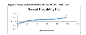
A normal probability plot on the relationship between annual inflation rate (AIR) and annual GDP growth (AGDPG) is presented in Figure 8. The figure depicts steady rise in comparative values over the fifty-six-year period. That is, from the 0.89th percentile through the 43.75th percentile to the 99.11th percentile. The foregoing notwithstanding, relatively flat distribution of comparative values over twenty-four-year period is observed from the 31.25th percentile through the 50.89th percentile to the 72.32nd percentile. Further, the distribution depicts steep rise in comparative values over the last fifteen-year period. That is, from the 74.11th percentile through the 91.96th percentile to the 99.11th percentile for the normal probability. Finally, we observe a sharp interval between the 0.89th percentile and the 2.68th percentile.
Generally, inflationary conditions in an economy may be open or suppressed. Conditions related to inflation may be described as suppressed when governments introduce price control mechanisms and other rationing devices to counter increased household consumption spending arising from increases in household incomes; which have the potential and often lead to price escalation.
The initiatives of governments in this regard help to salvage inflationary conditions from degenerating into embarrassing economic situations (Dutta, n.d.). Examples include the record of hyperinflation in the ensuing global economies in prior and recent years: Weimar Germany, Poland, Austria, Hungary, Venezuela and Zimbabwe. As a reiteration, data in Table 1; and Figures 3 and 4 affirm Ghana recorded hyperinflation during seven fiscal periods from 1965 through 2020, though the inflationary rates at issue did not compare with the astronomical rates recorded by the above-listed six economies. Ghana’s galloping inflation rates were recorded during the following fiscal periods: 1976 = 56.08%; 1978 = 73.09%; 1979 = 54.44%; 1980 = 50.07%; 1981 = 116.50%; 1983 = 122.87%; and 1995 = 59.46%.
Statistical test results for parameters of the regression model is presented in Table 6. Data on the coefficients, standard error, test statistic, significance, and confidence intervals for the coefficients are shared in the table. The coefficients in the table hint us on the contribution of the independent research variable (annual inflation) to the regression model. Generally, positive coefficient connotes positive relationship between the independent variable and the dependent variable; whereas negative value is indicative of negative relationship between the two variables.
We observe positive coefficient value for results from the statistical tests presented in Table 6. The foregoing implies positive relationship exists between annual inflation and annual GDP growth. Results from the statistical analysis support Grier and Grier (as cited in Zivkov et al.) who affirmed the absence of theoretical consensus on definitive influence of inflation on GDP growth; varied forms of empirical findings depict either positive, negative or neutral effect of average inflation on GDP growth.
Table 6: Model Parameters

Further, relationship between the two variables is significant (p = 0.006, p < 0.05). This implies annual inflation has significant influence on annual GDP growth. A consensus view of some economists is persistent price increase could lead to economic stimulation; and spur the economy on to higher growth rates. However, economic growth rates engineered by rising inflationary levels is not sustainable in the medium- and long-term. Nonetheless, GDP growth recorded by economies may be sustainable when the growth rates are influenced by mild or creeping inflationary levels.
The statistical output validates the influence of inflation on GDP growth; potential of prevailing macroeconomic conditions to inflate the Ghanaian economy; urgent need for a mix of more expansionary macroeconomic policy to ensure economic stimulation without necessarily escalating inflation; potential of inflation to threaten growth of the Ghanaian economy; and the need for inflation control to remain one of the top priorities among targets for monetary and fiscal policies. The statistical results affirm, high inflationary level has the potential to create distortions within the Ghanaian economy; and the distortions created thereof could be compared with unsatisfactory inducements shaped by unacceptable tax arrangements.
Generally, a large t-test value connotes the existence of large difference between sample groups, vice versa. The small t-test value in Table 6 is indicative of the similarity of sampled data for the independent research variable (annual inflation) and the dependent research variable (annual GDP growth). Moreover, magnitude of the t-test (p = 0.006, p < 0.05) avers significant influence of the independent research variable on the dependent research variable. A standard error is identified with the coefficients in the table. The standard error is indicative of the extent to which the coefficients would vary in different research samples (Field, 2009).
The probability that a parameter would fall between a pair of values around the mean is measured by the confidence interval. Stated differently, confidence interval values affirm the extent or level of uncertainty; or certainty in a method of sampling (Hayes, 2021). Available data in Table 6 depict the respective lower and upper 95% confidence interval values for the Intercept (0.036866472 and 0.06883528); and X Variable 1 (-0.101943691 and -0.0175559).
When inflation is anticipated, its redistributive effects on wealth and income tend to be minimal. Anticipated inflation enables individuals, businesses and economies to map-out cogent strategies to cope with inflation and its attendant effects. Suppose policymakers are able to anticipate annual inflation rate correctly. This would create the enabling environment for individuals, businesses and investors to develop strategies that would provide the needed protection against the threats of inflation including losses. Should inflation be expected to rise by 7%, labour would demand 7% increase in wage-rate; and lenders would demand a percentage increase in lending rates from borrowers. Firms would also set new prices to reflect the anticipated inflation rate (Dutta, n.d.).
Dutta (n.d.) posited, overall, the redistributive burden of inflation is lessened when the whole society strives to cope and live with inflation. Realisation of the foregoing is challenged by the inadequacies inherent in effective anticipation of inflation and its related episode. Thus, perfect anticipation of inflation cannot be guaranteed.
Moreover, adjustments required with the new inflationary situations may not be compatible with all categories of people; suggesting possible occurrence of adverse redistributive effects. Should individuals’ expectations from future price increase become stronger, they would hold less liquid money; and spend more or invest more in the current financial year. This renders inflation costly to society as less liquidity money is made available for spending during future financial periods.
Test of Assumptions
In order to determine linearity of the relationship between the independent variable (annual inflation) and the dependent variable (annual GDP growth), statistical tests were conducted. Further, statistical tests were conducted to measure the variance in residual values. Minimising the level of residuals or errors underlies the objectives of regression models. Due to the foregoing, residual diagnostics tend to play critical role in diagnostics tests related to economic modelling.
Generally, ideal error terms are expected to be white noise; implying they must be independent and identically distributed (iid). Fortunately, residual diagnostics facilitate our determination of whether or not the error terms in a given set of variables are independent and identically distributed (Shrestha & Bhatta, 2018).
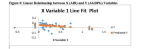
The statistical outputs on residuals are presented in Figures 9 and 10; and Table 7. The plots in Figure 9 depict the residuals scattered around the predicted variable on a horizontal or straight line. This asserts relationship between the independent research variable, annual inflation rate (AIR); and the dependent research variable, annual GDP growth (AGDPG), is linear; it implies the linear regression model fits the analysis.
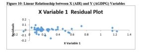
Moreover, the residual plot in Figure 10 depicts the independent variable (annual inflation rate) on the horizontal axis and the residuals on the vertical axis. The residual plots in the figure show a random pattern. That is, the points are randomly dispersed around the horizontal axis, affirming appropriateness of the linear model for the research data. Stated differently, the scatter plots in Figures 9 and 10 affirm fitness and appropriateness of the linear regression model for the current research.
Homoscedasticity tests remain one of the major test methods for residual diagnostics. Generally, residual diagnostic tests provide reliable information which facilitates our ability to determine the robustness of estimated coefficients. The residual values in Table 7 allow us to test the homoscedasticity of the model. That is, whether or not the residual values at each level of the independent variable depict constant variance; or homogeneity of variance. Residuals in the table show constant variance values. This implies the assumption of homoscedasticity is met.
Further, data in Figures 9 and 10 indicate relationship between the X and Y variables were measured at the interval level and beyond; while variability of the dependent research variable (annual GDP growth) was not constrained. The foregoing analysis indicates most of the assumptions have been met; this renders the regression model fit and appropriate for the current research.
Table 7: Predicted Y Values and Residual Values for Variable X
| Observation | Predicted Y | Residuals | Standard Residuals |
| 1 | 0.046905771 | -0.038105771 | -0.913960554 |
| 2 | 0.048560841 | 0.016239159 | 0.38949353 |
| 3 | 0.048184417 | 0.014415583 | 0.345755359 |
| 4 | 0.045459825 | 0.035940175 | 0.862019092 |
| 5 | 0.042424535 | -0.007924535 | -0.190068648 |
| 6 | 0.042603784 | -0.020803784 | -0.498975297 |
| 7 | 0.043595631 | -0.014595631 | -0.35007378 |
| 8 | 0.045878074 | 0.027221926 | 0.652913352 |
| 9 | 0.048590715 | 0.044309285 | 1.062750796 |
| 10 | 0.047634718 | 0.092865282 | 2.227358282 |
| 11 | 0.046451672 | 0.032548328 | 0.780666211 |
| 12 | 0.041349038 | 0.007050962 | 0.169116139 |
| 13 | 0.042980208 | 0.048519792 | 1.163739111 |
| 14 | 0.046439722 | -0.002939722 | -0.070508748 |
| 15 | 0.046326198 | 0.017673802 | 0.423903201 |
| 16 | 0.043816706 | 0.015183294 | 0.364168784 |
| 17 | 0.045310451 | 0.010689549 | 0.256387053 |
| 18 | 0.036915602 | 0.015084398 | 0.361796761 |
| 19 | 0.043995955 | 0.001004045 | 0.024081853 |
| 20 | 0.033187214 | 0.006812786 | 0.163403533 |
| 21 | 0.0377999 | -0.0007999 | -0.019185457 |
| 22 | 0.045435925 | -0.001435925 | -0.034440432 |
| 23 | 0.044115455 | 0.002884545 | 0.06918534 |
| 24 | 0.036186655 | 0.005813345 | 0.139432119 |
| 25 | 0.025031365 | 0.020968635 | 0.502929215 |
| 26 | 0.017323639 | 0.023776361 | 0.570272047 |
| 27 | 0.037991099 | -0.004991099 | -0.119710675 |
| 28 | 0.037937324 | 0.010562676 | 0.253344019 |
| 29 | 0.046840046 | -0.008040046 | -0.192839161 |
| 30 | 0.042077986 | 0.010722014 | 0.257165716 |
| 31 | 0.030588097 | 0.002711903 | 0.065044534 |
| 32 | 0.037781975 | 0.013118025 | 0.314633651 |
| 33 | 0.034113336 | 0.022186664 | 0.53214343 |
| 34 | 0.029058502 | 0.018841498 | 0.451910182 |
| 35 | 0.038170348 | 0.013829652 | 0.331701887 |
| 36 | 0.046690671 | 0.004209329 | 0.100960043 |
| 37 | 0.029148127 | 0.057351873 | 1.375575108 |
| 38 | -0.02056372 | -0.025036284 | -0.60049109 |
| 39 | 0.039526669 | -0.108726669 | -2.607791016 |
| 40 | -0.01675765 | -0.018242347 | -0.437539644 |
| 41 | 0.022934146 | -0.018234146 | -0.437342961 |
| 42 | 0.02032308 | -0.04542308 | -1.089464988 |
| 43 | 0.00917974 | 0.07562026 | 1.81373932 |
| 44 | -0.01672778 | 0.039427778 | 0.945668683 |
| 45 | 0.019343183 | -0.054643183 | -1.310607622 |
| 46 | 0.035033483 | -0.159333483 | -3.82158701 |
| 47 | 0.042018236 | 0.026481764 | 0.635160686 |
| 48 | 0.04228711 | -0.01348711 | -0.323486092 |
| 49 | 0.046834071 | -0.071734071 | -1.720529723 |
| 50 | 0.047138795 | 0.005061205 | 0.121392156 |
| 51 | 0.051040458 | 0.046159542 | 1.107128919 |
| 52 | 0.048477191 | 0.011622809 | 0.278771139 |
| 53 | 0.048136617 | -0.044436617 | -1.065804841 |
| 54 | 0.057881811 | -0.027081811 | -0.649552721 |
| 55 | 0.044940002 | -0.087540002 | -2.099632341 |
| 56 | 0.037053027 | -0.023353027 | -0.560118453 |
Report on P -Value and Confidence Interval
Data in Table 6 depict respective P-value of 0.006 and coefficients value of 0.05974981. These values are significant at Alpha level ɑ = 0.05. Data in the table further show confidence interval of -0.101943691 and -0.0175559. The Alpha level, a priori, for this study is ɑ = 0.05. The inference is there is 5% probability that we would be wrong; and there is 5% likelihood that the population mean would not fall within the interval (Ashley et al.; Bowerman & O’Connell, 1990; Frankfort-Nachmias and Nachmias, 2008). However, we are 95% (100% – 5%) certain our conclusions would be right. Again, the Microsoft Excel output in Table 5 shows degree of freedom (between) of 1 (2 – 1 = 1); degrees of freedom (within) of 54 (56 – 2 = 54); total degrees of freedom (df) of 55 (56 – 1 = 55), and an F-value of 8.06028894. These values could be interpreted as:
F (1, 54) = 8.06028894, p < 0.05, two-tailed.
Interpretation and Rejection of Null Hypothesis
Results from the foregoing analysis indicate inflation has significant impact on GDP growth. Therefore, we reject the null hypothesis (Ho: µ1 = µ2) which states, annual inflation has no strong effect on annual GDP growth within the Ghanaian economy; and accept the alternative hypothesis (H1: µ1 ≠ µ2) which states, annual inflation has strong effect on annual GDP growth within the Ghanaian economy.
Table 1: Historical Data on Ghana’s Inflation, GDP & GDP Growth Rates – 1960 – 2020
| Year | Annual Inflation Rate | Annual Inflation Change | GDP Value in US$ Billions | GDP Growth Rate |
| 2020 | 9.95% | 2.77% | 67.34 | 0.88% |
| 2019 | 7.18% | -0.63% | 66.98 | 6.48% |
| 2018 | 7.81% | -4.56% | 65.56 | 6.26% |
| 2017 | 12.37% | -5.08% | 59 | 8.14% |
| 2016 | 17.45% | 0.30% | 55.01 | 3.45% |
| 2015 | 17.15% | 1.66% | 48.56 | 2.18% |
| 2014 | 15.49% | 3.82% | 53.66 | 2.90% |
| 2013 | 11.67% | 4.54% | 62.41 | 7.31% |
| 2012 | 7.13% | -1.60% | 41.27 | 9.29% |
| 2011 | 8.73% | -1.98% | 39.34 | 14.05% |
| 2010 | 10.71% | -8.54% | 32.20 | 7.90% |
| 2009 | 19.25% | 2.73% | 25.98 | 4.84% |
| 2008 | 16.52% | 5.79% | 28.53 | 9.15% |
| 2007 | 10.73% | -0.18% | 24.76 | 4.35% |
| 2006 | 10.92% | -4.20% | 20.41 | 6.40% |
| 2005 | 15.12% | 2.49% | 10.73 | 5.90% |
| 2004 | 12.62% | -14.05% | 8.88 | 5.60% |
| 2003 | 26.67% | 11.86% | 7.63 | 5.20% |
| 2002 | 14.82% | -18.09% | 6.17 | 4.50% |
| 2001 | 32.91% | 7.71% | 5.31 | 4.00% |
| 2000 | 25.19% | 12.78% | 4.98 | 3.70% |
| 1999 | 12.41% | -2.22% | 7.72 | 4.40% |
| 1998 | 14.62% | -13.26% | 7.48 | 4.70% |
| 1997 | 27.89% | -18.68% | 6.89 | 4.20% |
| 1996 | 46.56% | -12.90% | 6.93 | 4.60% |
| 1995 | 59.46% | 34.59% | 6.47 | 4.11% |
| 1994 | 24.87% | -0.09% | 5.44 | 3.30% |
| 1993 | 24.96% | 14.90% | 5.97 | 4.85% |
| 1992 | 10.06% | -7.98% | 6.41 | 3.88% |
| 1991 | 18.03% | -19.23% | 6.60 | 5.28% |
| 1990 | 37.26% | 12.04% | 5.89 | 3.33% |
| 1989 | 25.22% | -6.14% | 5.25 | 5.09% |
| 1988 | 31.36% | -8.46% | 5.20 | 5.63% |
| 1987 | 39.82% | 15.25% | 5.07 | 4.79% |
| 1986 | 24.57% | 14.26% | 5.73 | 5.20% |
| 1985 | 10.31% | -29.36% | 4.50 | 5.09% |
| 1984 | 39.67% | -83.21% | 4.41 | 8.65% |
| 1983 | 122.87% | 100.58% | 4.06 | -4.56% |
| 1982 | 22.30% | -94.21% | 4.04 | -6.92% |
| 1981 | 116.50% | 66.43% | 4.22 | -3.50% |
| 1980 | 50.07% | -4.37% | 4.45 | 0.47% |
| 1979 | 54.44% | -18.65% | 4.02 | -2.51% |
| 1978 | 73.09% | -43.36% | 3.66 | 8.48% |
| 1977 | 116.45% | 60.37% | 3.19 | 2.27% |
| 1976 | 56.08% | 26.26% | 2.77 | -3.53% |
| 1975 | 29.82% | 11.69% | 2.81 | -12.43% |
| 1974 | 18.13% | 0.45% | 2.89 | 6.85% |
| 1973 | 17.68% | 7.62% | 2.47 | 2.88% |
| 1972 | 10.07% | 0.51% | 2.11 | -2.49% |
| 1971 | 9.56% | 6.53% | 2.42 | 5.22% |
| 1970 | 3.03% | -4.29% | 2.22 | 9.72% |
| 1969 | 7.32% | -0.58% | 1.96 | 6.01% |
| 1968 | 7.89% | 16.32% | 1.67 | 0.37% |
| 1967 | -8.42% | -21.66% | 1.75 | 3.08% |
| 1966 | 13.24% | -13.21% | 2.13 | -4.26% |
| 1965 | 26.44% | -13.21% | 2.05 | 1.37% |
| 1964 | – | – | 1.73 | 2.21% |
| 1963 | – | – | 1.54 | 4.41% |
| 1962 | – | – | 1.38 | 4.11% |
| 1961 | – | – | 1.30 | 3.43% |
| 1960 | – | – | 1.22 | – |
Sources: MacroTrends (2020a & 2020b); World Bank (2021b, d, & g)
Figure 1: Statistics on Annual GDP Growth Rate – 1961 – 2020
| Mean | 0.036108197 |
| Standard Error | 0.005519385 |
| Median | 0.044 |
| Mode | 0.052 |
| Standard Deviation | 0.043107773 |
| Sample Variance | 0.00185828 |
| Kurtosis | 2.874190128 |
| Skewness | -1.14076322 |
| Range | 0.2648 |
| Minimum | -0.1243 |
| Maximum | 0.1405 |
| Sum | 2.2026 |
| Count | 61 |
| Largest(1) | 0.1405 |
| Smallest(1) | -0.1243 |
| Confidence Level (95.0%) | 0.011040413 |
Figure 2: Statistics on Annual Change in Inflation Rate – 1965 – 2020
| Mean | -0.005308929 |
| Standard Error | 0.037563978 |
| Median | -0.0038 |
| Mode | -0.1321 |
| Standard Deviation | 0.281103068 |
| Sample Variance | 0.079018935 |
| Kurtosis | 5.576938747 |
| Skewness | 0.095525854 |
| Range | 1.9479 |
| Minimum | -0.9421 |
| Maximum | 1.0058 |
| Sum | -0.2973 |
| Count | 56 |
| Largest(1) | 1.0058 |
| Smallest(1) | -0.9421 |
| Confidence Level (95.0%) | 0.075279893 |
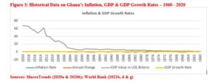
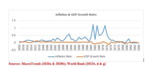
Figure 4: Trend in Inflation and GDP Growth Rates in Ghana – 1961 – 2020
Authors’ Note
The above write-up was extracted from recent Publication on “Nexus between Inflation and GDP Growth” by Ashley, Andani, Sackey and Ackah (2024) in the International Journal of Business and Management (IJBM). DOI No.: 10.24940/theijbm/2024/v12/i1/BM2401-016
: A Strategic Shift from traditional methods")


: A Strategic Shift from traditional methods")


